2021.05.24 - [딥러닝관련/기초 이론] - 신경망 정리 6 (경사법, 경사 하강법)
신경망 정리 6 (경사법, 경사 하강법)
경사법(gradient method) 기울기를 활용해 함수의 손실 함수의 최솟값(또는 가능한 한 작은 값)을 찾으려는 것이 경사법 그러나, 기울기가 가리키는 곳에 정말 함수의 최솟값이 있는지, 즉 그쪽이 정
better-tomorrow.tistory.com
위 내용에 이어 학습 알고리즘을 구현한다.
신경망 학습의 절차
1단계 - 미니배치
훈련 데이터 중 일부를 무작위로 가져온다. 이렇게 선별한 데이터를 미니배치라 하며, 그 미니배치의 손실 함수 값을 줄이는 것을 목표로 한다.
2단계 - 기울기 산출
미니배치의 손실 함수 값을 줄이기 위해 각 가중치 매개변수의 기울기를 구한다. 기울기는 손실 함수의 값을 가장 작게 하는 방향을 제시
3단계 - 매개변수 갱신
가중치 매개변수를 기울기 방향으로 아주 조금 갱신
4단계 - 반복
1~3단계를 반복한다.
이때 데이터를 미니배치로 무작위로 선정하기 때문에 확률적 경사 하강법(stochastic gradient descent, SGD)라고 불린다.
'확률적으로 무작위로 골라낸 데이터'에 대해 수행하는 경사 하강법이라는 의미
MNIST로 은닉층이 1개인 네트워크를 대상으로 MNIST 데이터셋 이용하여 구현
구현은 참고용으로만 확인
import sys, os
import numpy as np

def sigmoid(x):
    return 1 / (1 + np.exp(-x))

def softmax(x):
    if x.ndim == 2:
        x = x.T
        x = x - np.max(x, axis=0)
        y = np.exp(x) / np.sum(np.exp(x), axis=0)
        return y.T

    x = x - np.max(x) # 오버플로 대책
    return np.exp(x) / np.sum(np.exp(x))

def numerical_gradient(f, x):
    h = 1e-4  # 0.0001
    grad = np.zeros_like(x)

    it = np.nditer(x, flags=['multi_index'], op_flags=['readwrite'])
    while not it.finished:
        idx = it.multi_index
        tmp_val = x[idx]
        x[idx] = float(tmp_val) + h
        fxh1 = f(x)  # f(x+h)

        x[idx] = tmp_val - h
        fxh2 = f(x)  # f(x-h)
        grad[idx] = (fxh1 - fxh2) / (2 * h)

        x[idx] = tmp_val  # 값 복원
        it.iternext()

    return grad

def cross_entropy_error(y, t):
    if y.ndim == 1:
        t = t.reshape(1, t.size)
        y = y.reshape(1, y.size)

    # 훈련 데이터가 원-핫 벡터라면 정답 레이블의 인덱스로 반환
    if t.size == y.size:
        t = t.argmax(axis=1)

    batch_size = y.shape[0]
    return -np.sum(np.log(y[np.arange(batch_size), t] + 1e-7)) / batch_size

def sigmoid_grad(x):
    return (1.0 - sigmoid(x)) * sigmoid(x)

class TwoLayerNet:

    def __init__(self, input_size, hidden_size, output_size, weight_init_std=0.01):
        # 가중치 초기화
        self.params = {}
        self.params['W1'] = weight_init_std * np.random.randn(input_size, hidden_size)
        self.params['b1'] = np.zeros(hidden_size)
        self.params['W2'] = weight_init_std * np.random.randn(hidden_size, output_size)
        self.params['b2'] = np.zeros(output_size)

    def predict(self, x):
        W1, W2 = self.params['W1'], self.params['W2']
        b1, b2 = self.params['b1'], self.params['b2']

        a1 = np.dot(x, W1) + b1
        z1 = sigmoid(a1)
        a2 = np.dot(z1, W2) + b2
        y = softmax(a2)

        return y

    # x : 입력 데이터, t : 정답 레이블
    def loss(self, x, t):
        y = self.predict(x)

        return cross_entropy_error(y, t)

    def accuracy(self, x, t):
        y = self.predict(x)
        y = np.argmax(y, axis=1)
        t = np.argmax(t, axis=1)

        accuracy = np.sum(y == t) / float(x.shape[0])
        return accuracy

    # x : 입력 데이터, t : 정답 레이블
    def numerical_gradient(self, x, t):
        loss_W = lambda W: self.loss(x, t)

        # 각 매개변수의 기울기
        grads = {}
        grads['W1'] = numerical_gradient(loss_W, self.params['W1'])
        grads['b1'] = numerical_gradient(loss_W, self.params['b1'])
        grads['W2'] = numerical_gradient(loss_W, self.params['W2'])
        grads['b2'] = numerical_gradient(loss_W, self.params['b2'])

        return grads

    def gradient(self, x, t):
        W1, W2 = self.params['W1'], self.params['W2']
        b1, b2 = self.params['b1'], self.params['b2']
        grads = {}

        batch_num = x.shape[0]

        # forward
        a1 = np.dot(x, W1) + b1
        z1 = sigmoid(a1)
        a2 = np.dot(z1, W2) + b2
        y = softmax(a2)

        # backward
        dy = (y - t) / batch_num
        grads['W2'] = np.dot(z1.T, dy)
        grads['b2'] = np.sum(dy, axis=0)

        da1 = np.dot(dy, W2.T)
        dz1 = sigmoid_grad(a1) * da1
        grads['W1'] = np.dot(x.T, dz1)
        grads['b1'] = np.sum(dz1, axis=0)

        return grads


"""
실행
"""

net = TwoLayerNet(input_size=784, hidden_size=100, output_size=10)

# params : 신경망에 필요한 매개변수가 모두 저장 -> 저장된 가중치는 예측 처리에서 사용
print(net.params['W1'].shape) # (784, 100)
print(net.params['b1'].shape) # (100,)
print(net.params['W2'].shape) # (100, 10)
print(net.params['b2'].shape) # (10,)

# 예측

x = np.random.rand(100, 784) # 더미 입력 (100장)
y = net.predict(x)

# grads 변수에는 params 변수에 대응하는 각 매개변수의 기울기가 저장

x = np.random.rand(100, 784)
t = np.random.rand(100, 10)

grads = net.numerical_gradient(x, t)

print(grads['W1'].shape) # (784, 100)
print(grads['b1'].shape) # (100,)
print(grads['W2'].shape) # (100, 10)
print(grads['b2'].shape) # (10)
미니배치 학습 구현
# coding: utf-8
import sys, os
sys.path.append(os.pardir) # 부모 디렉터리의 파일을 가져올 수 있도록 설정
import numpy as np
import matplotlib.pyplot as plt
from dataset.mnist import load_mnist
# 데이터 읽기
(x_train, t_train), (x_test, t_test) = load_mnist(normalize=True, one_hot_label=True)
def sigmoid(x):
return 1 / (1 + np.exp(-x))
def cross_entropy_error(y, t):
if y.ndim == 1:
t = t.reshape(1, t.size)
y = y.reshape(1, y.size)
# 훈련 데이터가 원-핫 벡터라면 정답 레이블의 인덱스로 반환
if t.size == y.size:
t = t.argmax(axis=1)
batch_size = y.shape[0]
return -np.sum(np.log(y[np.arange(batch_size), t] + 1e-7)) / batch_size
def softmax(x):
if x.ndim == 2:
x = x.T
x = x - np.max(x, axis=0)
y = np.exp(x) / np.sum(np.exp(x), axis=0)
return y.T
x = x - np.max(x) # 오버플로 대책
return np.exp(x) / np.sum(np.exp(x))
def numerical_gradient(f, x):
h = 1e-4 # 0.0001
grad = np.zeros_like(x)
it = np.nditer(x, flags=['multi_index'], op_flags=['readwrite'])
while not it.finished:
idx = it.multi_index
tmp_val = x[idx]
x[idx] = float(tmp_val) + h
fxh1 = f(x) # f(x+h)
x[idx] = tmp_val - h
fxh2 = f(x) # f(x-h)
grad[idx] = (fxh1 - fxh2) / (2 * h)
x[idx] = tmp_val # 값 복원
it.iternext()
return grad
def sigmoid_grad(x):
return (1.0 - sigmoid(x)) * sigmoid(x)
class TwoLayerNet:
def __init__(self, input_size, hidden_size, output_size, weight_init_std=0.01):
# 가중치 초기화
self.params = {}
self.params['W1'] = weight_init_std * np.random.randn(input_size, hidden_size)
self.params['b1'] = np.zeros(hidden_size)
self.params['W2'] = weight_init_std * np.random.randn(hidden_size, output_size)
self.params['b2'] = np.zeros(output_size)
def predict(self, x):
W1, W2 = self.params['W1'], self.params['W2']
b1, b2 = self.params['b1'], self.params['b2']
a1 = np.dot(x, W1) + b1
z1 = sigmoid(a1)
a2 = np.dot(z1, W2) + b2
y = softmax(a2)
return y
# x : 입력 데이터, t : 정답 레이블
def loss(self, x, t):
y = self.predict(x)
return cross_entropy_error(y, t)
def accuracy(self, x, t):
y = self.predict(x)
y = np.argmax(y, axis=1)
t = np.argmax(t, axis=1)
accuracy = np.sum(y == t) / float(x.shape[0])
return accuracy
# x : 입력 데이터, t : 정답 레이블
def numerical_gradient(self, x, t):
loss_W = lambda W: self.loss(x, t)
grads = {}
grads['W1'] = numerical_gradient(loss_W, self.params['W1'])
grads['b1'] = numerical_gradient(loss_W, self.params['b1'])
grads['W2'] = numerical_gradient(loss_W, self.params['W2'])
grads['b2'] = numerical_gradient(loss_W, self.params['b2'])
return grads
def gradient(self, x, t):
W1, W2 = self.params['W1'], self.params['W2']
b1, b2 = self.params['b1'], self.params['b2']
grads = {}
batch_num = x.shape[0]
# forward
a1 = np.dot(x, W1) + b1
z1 = sigmoid(a1)
a2 = np.dot(z1, W2) + b2
y = softmax(a2)
# backward
dy = (y - t) / batch_num
grads['W2'] = np.dot(z1.T, dy)
grads['b2'] = np.sum(dy, axis=0)
da1 = np.dot(dy, W2.T)
dz1 = sigmoid_grad(a1) * da1
grads['W1'] = np.dot(x.T, dz1)
grads['b1'] = np.sum(dz1, axis=0)
return grads
network = TwoLayerNet(input_size=784, hidden_size=50, output_size=10)
# 하이퍼파라미터
iters_num = 10000 # 반복 횟수를 적절히 설정한다.
train_size = x_train.shape[0] # 60,000장
batch_size = 100 # 미니배치 크기
learning_rate = 0.1
train_loss_list = []
train_acc_list = []
test_acc_list = []
# 1에폭당 반복 수
iter_per_epoch = max(train_size / batch_size, 1) # 60000 / 100
for i in range(iters_num):
# 미니배치 획득
batch_mask = np.random.choice(train_size, batch_size) # 이미지 random 선택
x_batch = x_train[batch_mask]
t_batch = t_train[batch_mask]
# 기울기 계산
# grad = network.numerical_gradient(x_batch, t_batch)
grad = network.gradient(x_batch, t_batch)
# 매개변수 갱신
for key in ('W1', 'b1', 'W2', 'b2'):
network.params[key] -= learning_rate * grad[key]
# 학습 경과 기록
loss = network.loss(x_batch, t_batch)
train_loss_list.append(loss)
# 1에폭당 정확도 계산
if i % iter_per_epoch == 0:
train_acc = network.accuracy(x_train, t_train)
test_acc = network.accuracy(x_test, t_test)
train_acc_list.append(train_acc)
test_acc_list.append(test_acc)
print("train acc, test acc | " + str(train_acc) + ", " + str(test_acc))
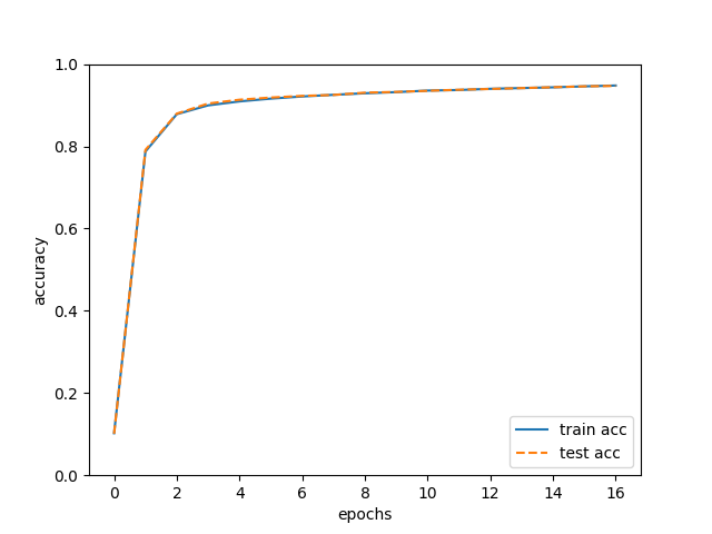
# 그래프 그리기
markers = {'train': 'o', 'test': 's'}
x = np.arange(len(train_acc_list))
plt.plot(x, train_acc_list, label='train acc')
plt.plot(x, test_acc_list, label='test acc', linestyle='--')
plt.xlabel("epochs")
plt.ylabel("accuracy")
plt.ylim(0, 1.0)
plt.legend(loc='lower right')
plt.show()
내용 참고
book.naver.com/bookdb/book_detail.nhn?bid=11492334
밑바닥부터 시작하는 딥러닝
직접 구현하고 움직여보며 익히는 가장 쉬운 딥러닝 입문서!『밑바닥부터 시작하는 딥러닝』은 라이브러리나 프레임워크에 의존하지 않고, 딥러닝의 핵심을 ‘밑바닥부터’ 직접 만들어보며
book.naver.com
'딥러닝관련 > 기초 이론' 카테고리의 다른 글
| 신경망 정리 9 (연쇄 법칙 chain rule) (0) | 2021.05.30 |
|---|---|
| 신경망 정리 8 (오차역전파법) (0) | 2021.05.29 |
| 기초 행렬 이론 정리 (0) | 2021.05.27 |
| 신경망 정리 6 (경사법, 경사 하강법) (0) | 2021.05.24 |
| 신경망 정리 5 (수치 미분, 편미분) (0) | 2021.05.23 |


